Measurement and signaling in the nonlocal world
Popular understanding of quantum mechanics usually focuses on three learning objectives:
- At small scales, particle properties (position, momentum, spin, etc.) are in superposition - they don’t have a definite value, but instead are “smeared” across multiple possible values.
- Measuring a superposed particle property makes it collapse probabilistically to a specific value. We don’t simply discover the property’s pre-existing value; rather the property is forced to take on a definite value by the act of measurement.
- Particles can be entangled, which means operations on one affect the other instantaneously across arbitrarily-large distances (known as nonlocality); however, this has restrictions and cannot be used for faster-than-light (FTL) communication.

This post focuses on the third point, specifically the part about FTL communication. There’s something called the “no-communication theorem” or “no-signaling principle” which shows that it’s impossible for us to use a pair of entangled particles as a FTL communication channel (much to the chagrin of many, many works of science fiction). Let’s be more precise: communication is a technical term which means I have some chosen bit (0 or 1) I can send to my counterpart on the other end of a channel. The channel doesn’t have to be perfect: all that matters is the receiver can discern the sent bit with probability better than a coin flip. A channel which enables the receiver to determine the correct bit only 51% of the time still involves communication, since we can re-send the same bit arbitrarily-many times to establish high levels of certainty of which bit was sent. The no-communication theorem says entangled particles, while indeed affecting one another in a FTL way, can never beat a coin flip when determining which bit was sent.
The no-communication theorem is obviously disheartening, so let’s stay in the Denial stage for a bit and poke around. Sending a full bit via a pair of entangled particles is, like many things humans want, too much to ask of the universe. Maybe there’s a hidden consolation prize, though? Clearly some kind of FTL interaction is taking place; surely it isn’t completely useless? Generations of clever scientists have considered this problem, and come up with very interesting scenarios where entanglement gives us FTL… coordination? Correlation? It’s difficult describe a phenomenon which isn’t communication, but it is something. Here we’ll learn just what that something is.
Preliminaries: entanglement and measurement
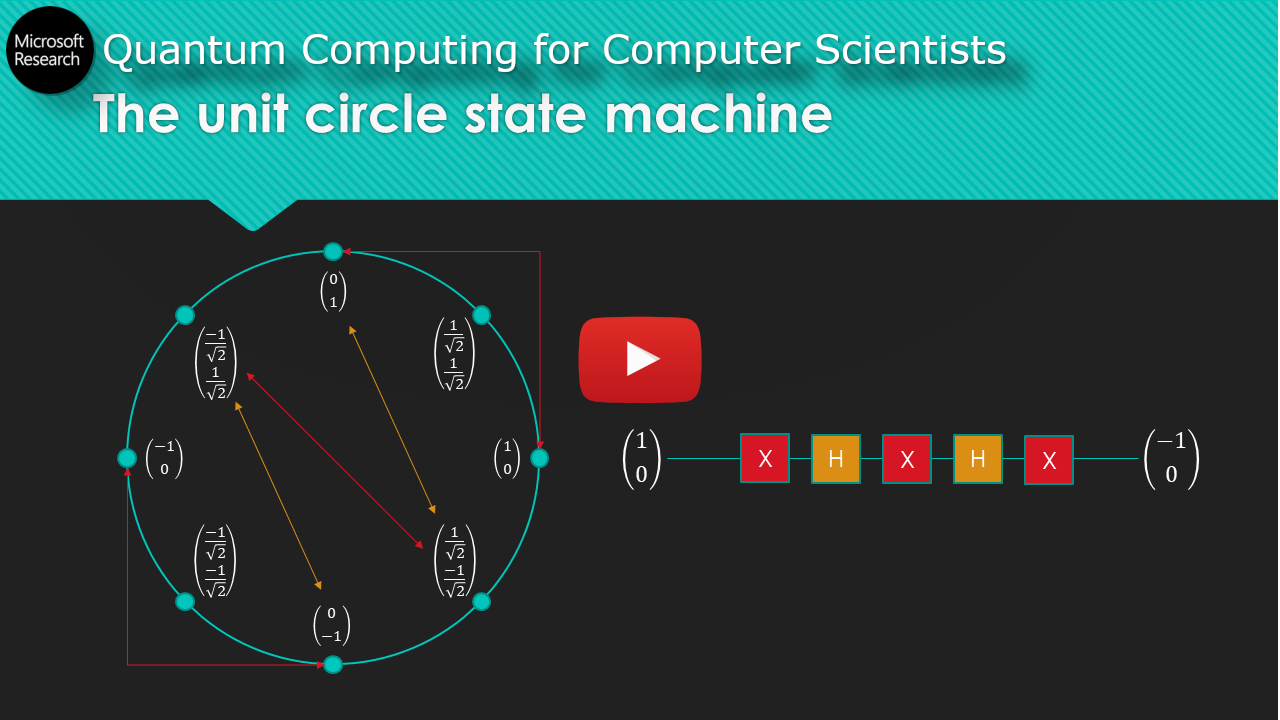
The rest of this post assumes basic familiarity with the bra-ket mathematical formalism of quantum computing; if you do not have this, you can watch a lecture I’ve created aimed at computer scientists here (slides: pdf, pptx):
Review of the actual vector values of the common quantum states \(|0\rangle\), \(|1\rangle\), \(|+\rangle\), and \(|-\rangle\): $$ |0\rangle = \begin{bmatrix} 1 \\ 0 \end{bmatrix}, |1\rangle = \begin{bmatrix} 0 \\ 1 \end{bmatrix}, |+\rangle = \begin{bmatrix} \frac{1}{\sqrt{2}} \\ \frac{1}{\sqrt{2}} \end{bmatrix}, |-\rangle = \begin{bmatrix} \frac{1}{\sqrt{2}} \\ \frac{-1}{\sqrt{2}} \end{bmatrix} $$
Here we’ll establish some knowledge required for the main event. Recall two qbits are entangled when you cannot factor their product state into the tensor product of two individual qbit states:
$$ |\Phi^+\rangle = \begin{bmatrix} \frac{1}{\sqrt{2}} \\ 0 \\ 0 \\ \frac{1}{\sqrt{2}} \end{bmatrix} \neq \begin{bmatrix} a \\ b \end{bmatrix} \otimes \begin{bmatrix} c \\ d \end{bmatrix} $$ Try to factor this! You can’t; you get a system of four equations with no solution.
If you were to measure this state in the computational basis (collapsing each qbit to \(|0\rangle\) or \(|1\rangle\), it will only ever collapse to \(|00\rangle\) or \(|11\rangle\) with equal probability. If you measure one of the qbits before the other, it instantaneously forces the other qbit into the same state as the first. So if you measure one qbit and it collapses to \(|0\rangle\), you know the other qbit also collapsed to \(|0\rangle\).
The computational basis is not the only way of measuring qbits; you can also measure in another basis called the sign basis:
After measuring in the sign basis, your qbit will be in state \(|+\rangle\) or \(|-\rangle\) instead of \(|0\rangle\) or \(|1\rangle\). These types of measurements are called projective measurements, because what we’re doing is projecting a quantum state onto one of the two measurement basis vectors:
In addition to the computational & sign bases, we can use any pair of orthonormal vectors as a basis for qbit measurement!
Something very curious happens if we measure our entangled qbit state in the sign basis - instead of collapsing to \(|00\rangle\) or \(|11\rangle\), it collapses to \(|++\rangle\) or \(|- - \rangle\)! In fact, regardless of the basis in which you measure, if one qbit collapses to a value then the other entangled qbit also collapses to that same value! This is a property called rotational invariance, and we make much use of it below.
There’s one more detail to cover, and that’s how to calculate the probability of collapse in these other measurement bases. A bit of high-school trigonometry does the trick:
The angle between the state vector and \(|+\rangle\) basis vector is \(\pi/8\) radians, and the angle between the state vector and \(|-\rangle\) basis vector is \(3\pi/8\) radians. The distance from the origin to point \(x\) is given by \(\cos(3\pi/8)=0.38\), and the distance from the origin to point \(y\) is given by \(\sin(3\pi/8)=0.92\). Square the absolute value of this distance to get the probability of collapse to that basis vector: \(0.85\) for \(|+\rangle\), and \(0.15\) for \(|-\rangle\).
A curious game
Consider a game involving two people, Alice and Bob. Alice is given a random bit \(X\) and Bob a random bit \(Y\). Alice then outputs a chosen bit \(A\) and Bob a chosen bit \(B\). Their objective? Satisfy the logical formula \(X \cdot Y = A \oplus B\). The catch? Alice and Bob cannot communicate.
Let’s break down this formula; here’s the truth table for \(X \cdot Y\):
| \(X\) | \(Y\) | \(X \cdot Y\) |
|---|---|---|
| 0 | 0 | 0 |
| 0 | 1 | 0 |
| 1 | 0 | 0 |
| 1 | 1 | 1 |
Here’s the truth table for \(A \oplus B\):
| \(A\) | \(B\) | \(A \oplus B\) |
|---|---|---|
| 0 | 0 | 0 |
| 0 | 1 | 1 |
| 1 | 0 | 1 |
| 1 | 1 | 0 |
Careful consideration of the above rules and truth tables gives rise to an important observation: Alice and Bob cannot possibly win the game every time. All they can do is pick an approach which maximizes their probability of success. The winning strategy is quite simple: Alice and Bob both always output \(0\), regardless of their input values. This gives them a 75% chance of winning; they’ll only lose in the case where both \(X\) and \(Y\) are \(1\). Proof omitted, this is the best possible classical strategy.
What if we bend the rules a little so Alice and Bob are each in possession of one half of a two-qbit entangled quantum state in addition to their random input bit? Something remarkable happens: a strategy exists which enables them to win 85% of the time instead of 75%! A 10% advantage doesn’t seem earth-shattering at first glance, but the implications are far-reaching (and exquisitely detailed in this Scholarpedia article). How does it work?
The high-level strategy has Alice and Bob measuring their entangled qbits in different bases depending on whether they’re given a \(0\) or a \(1\). They use the results of those measurements to decide whether to output \(0\) or \(1\) themselves. Amazingly, through clever choice of measurement bases we can ensure our \(\theta\) (the angle between the state vector and one of the measurement basis vectors) always equals \(\pi/8\) for the outcome we want. What is \(\cos^2(\pi/8)\)? Approximately \(0.85\), of course!
Let’s look at Alice’s strategy first:
| If Alice receives | she measures in the | and if she gets | she outputs |
|---|---|---|---|
| 0 | computational basis | \(|0\rangle\) | 0 |
| 0 | computational basis | \(|1\rangle\) | 1 |
| 1 | sign basis | \(|+\rangle\) | 0 |
| 1 | sign basis | \(|-\rangle\) | 1 |
Simple so far? Bob’s strategy is a bit more complicated. If he receives a \(0\), he measures in the computational basis rotated \(\pi/8\) radians counter-clockwise around the unit circle (henceforth called the \(\pi/8\) basis):
If Bob receives a \(1\), he measures in the computational basis rotated \(\pi/8\) radians clockwise around the unit circle (henceforth called the \(-\pi/8\) basis):
As marked on the diagrams, Bob outputs a \(0\) if his measurement results in the vector closest to horizontal. If it results in the vector closest to vertical, he outputs a \(1\). Curiously, these strategies result in an 85% chance of satisfying the logical formula \(X \cdot Y = A \oplus B\)! It also works regardless of who measures their qbit first, ensuring no communication is required between Alice and Bob.
Let’s take an example and see how it plays out. Consider the case when both Alice and Bob receive \(1\) as input. Recall this is the case that trips up the classical strategy - we want Alice OR Bob to output \(1\) here, but not both. Say Alice measures her qbit first, in the sign basis since she received a \(1\) as input. She has a 50% chance of measuring \(|+\rangle\), and a 50% chance of measuring \(|-\rangle\). Whichever outcome she measured, Bob’s qbit is now also in that state:
Bob will then measure his qbit in the \(-\pi/8\) basis, since he also received a \(1\) as input:
Here’s how the cases break down:
| If Alice outputs | then Bob’s qbit is | so Bob outputs 0 with probability | and 1 with probability |
|---|---|---|---|
| 0 | \(|+\rangle\) | \(\cos^2(3\pi/8)=0.15\) | \(\sin^2(3\pi/8)=0.85\) |
| 1 | \(|-\rangle\) | \(\cos^2(-\pi/8)=0.85\) | \(\sin^2(-\pi/8)=0.15\) |
We see that in the case where Alice measured \(|+\rangle\) (and will thus output \(0\)) Bob has an 85% chance of outputting \(1\), and in the case where Alice measured \(|-\rangle\) (and will thus output \(1\)) Bob has an 85% chance of outputting \(0\). So, there’s an 85% chance overall that exactly one of Alice and Bob will output \(1\), satisfying \(X \cdot Y = A \oplus B\)! You can similarly analyze the cases where the inputs are \(00\), \(01\), and \(10\) (or when Bob measures before Alice) and see they always give an 85% chance of success. Amazing!
Applications and implications
The game described above is called the CHSH game, after the initials of the physicists who first proposed it (John Clauser, Michael Horne, Abner Shimony, and Richard Holt). It’s a bit of a head-scratcher how we can actually make use of it. We might consider two space admirals fighting separate space battles separated by light-years; the outcome of those battles is either a loss (input 0) or a win (input 1), and if they both win then one of them needs to proceed to a further objective (output 1) while the other returns home (output 0). Or something. Or a quantum twist on the prisoner’s dilemma. I’m sure others have put more thought & imagination into this than I have.
One concrete application of these nonlocal games as they’re called (there are others beyond the CHSH game; see Consequences and Limits of Nonlocal Strategies by Cleve et al.) is device-independent quantum cryptography; see also this QCSE question. The basic idea is you’ll be able to execute cryptographic operations on untrusted quantum computers, by using nonlocal games to test that they’re honestly using quantum phenomena.
The implications of the CHSH game are extreme. They form the core of Bell’s theorem, which has been called “the most profound discovery of science” and states that no physical theory of local hidden variables can ever reproduce all the predictions of quantum mechanics. It’s all about locality, or rather how locality isn’t true - quantum entanglement really is faster-than-light, and doesn’t have any obvious medium through which it works! Before Bell’s theorem, people suspected there was some mechanism whereby entangled particles decided how they would collapse at time of entanglement, not at time of measurement, then carried that decision (a “hidden variable”) with them until they were measured. The CHSH game blows this theory out of the water. Consider the following argument:
- If particles decide at time of entanglement how they will collapse, they must carry within them some information (the local hidden variable). This information can be represented as a string of classical bits.
- Since the information is sufficient to completely describe the way in which the entangled qbits collapse, Alice and Bob could, if given access to that same string of classical bits, emulate the behavior of their qbits.
- If Alice and Bob could emulate the behavior of their qbits, they could implement the quantum strategy with purely classical methods using the string of classical bits. Thus, there must exist some classical strategy giving an 85% success rate with some string of bits as input.
- However, there exists no string of bits which enables a classical strategy with success rate above 75% (proof omitted, just take my word for it); by contradiction, the behavior of entangled particles is not reducible to a string of bits (local hidden variable) and thus the entangled particles must instantaneously affect one another at time of measurement.
This isn’t just theoretical - the experiments have been done and the numbers are in. Nonlocality is fundamental to how our universe works. For a detailed treatment of this topic, see the Scholarpedia or SEP articles.
In the end, the CHSH game is to me paradigmatic of the subtlety of quantum mechanics - and how exploring that subtlety yields rich rewards in a way no other field seems to match.
Implementation in Q#
It’s easy to distrust abstract reasoning, especially in unintuitive realms like probability; unless you’re a hardened mathematician, you want to see the results! To that end, I wrote up the CHSH game in Q#, Microsoft’s quantum language. The game is played 10,000 times with random input bits given to Alice and Bob (plus another random bit controlling who measures first) to see whether they really win 85% of the time vs. 75% of the time with the classical strategy. Lo and behold:
$ dotnet run
Classical success rate: 0.7474
Quantum success rate: 0.8592
SPOOKY
Really should have published this blog post on/around Halloween.
You can find the source code here. The code is very simple except for one thing: measurement. Here’s how we specify measurement in common bases like the computational or sign bases:
// Two equivalent methods of measuring in the computational basis
Measure([PauliZ], [qubit]);
M(qubit);

// Measuring in the sign basis
Measure([PauliX], [qubit]);
The PauliZ and PauliX parameters refer to the Pauli matrices:
$$ \sigma_z = \begin{bmatrix} 1 & 0 \\ 0 & -1 \end{bmatrix}, \sigma_x = \begin{bmatrix} 0 & 1 \\ 1 & 0 \end{bmatrix} $$
It seems odd to specify measurement bases with matrices, but the two bases we want here (the computational and sign bases) are the eigenvectors of these matrices. Recall an eigenvector of a matrix is a vector which, when multiplied by the matrix, is changed only by a constant multiplicative factor (called an eigenvalue):
$$ \sigma_z|0\rangle = \begin{bmatrix} 1 & 0 \\ 0 & -1 \end{bmatrix} \begin{bmatrix} 1 \\ 0 \end{bmatrix} = \begin{bmatrix} 1 \\ 0 \end{bmatrix} = 1|0\rangle $$ $$ \sigma_z|1\rangle = \begin{bmatrix} 1 & 0 \\ 0 & -1 \end{bmatrix} \begin{bmatrix} 0 \\ 1 \end{bmatrix} = \begin{bmatrix} 0 \\ -1 \end{bmatrix} = -1|1\rangle $$ $$ \sigma_x|+\rangle = \begin{bmatrix} 0 & 1 \\ 1 & 0 \end{bmatrix} \begin{bmatrix} \frac{1}{\sqrt{2}} \\ \frac{1}{\sqrt{2}} \end{bmatrix} = \begin{bmatrix} \frac{1}{\sqrt{2}} \\ \frac{1}{\sqrt{2}} \end{bmatrix} = 1|+\rangle $$ $$ \sigma_x|-\rangle = \begin{bmatrix} 0 & 1 \\ 1 & 0 \end{bmatrix} \begin{bmatrix} \frac{1}{\sqrt{2}} \\ \frac{-1}{\sqrt{2}} \end{bmatrix} = \begin{bmatrix} \frac{-1}{\sqrt{2}} \\ \frac{1}{\sqrt{2}} \end{bmatrix} = -1|-\rangle $$
It is thus convenient to identify common measurement bases in this way; we call the matrices observables. You can think of these matrices as corresponding in some way to the measurement device, which forces the quantum state to collapse to one of its eigenvectors and displays the eigenvalue to the user - perhaps deflecting a needle in the positive direction if the state collapsed to the eigenvector with eigenvalue 1, and deflecting a needle in the negative direction if the state collapsed to the eigenvector with eigenvalue -1.
Things are slightly more complicated when measuring in Bob’s nonstandard bases. To measure in the π/8 basis, we do the following:
- Rotate the quantum state π/8 radians clockwise around the unit circle
- Measure in the computational basis
This is a bit strange; here’s what we’re doing graphically:
This method is weird, but it works. To measure in the -π/8 basis, we do something similar:
- Rotate the quantum state π/8 radians counter-clockwise around the unit circle
- Measure in the computational basis
Again, here’s the graphical representation of what we’re doing:
In terms of actual Q# code, we write this as follows:
// Measure in π/8 basis
let rotation = -2.0 * PI() / 8.0;
Ry(rotation, qubit);
return M(qubit);

// Measure in -π/8 basis
let rotation = 2.0 * PI() / 8.0;
Ry(rotation, qubit);
return M(qubit);
We use the Ry operator to rotate the quantum state in the unit circle plane.
Credit to Mariia Mykhailova from the Microsoft Quantum team for explaining how to do this!
Resources and further reading
-
Dr. Umesh Vazirani’s Quantum Mechanics & Quantum Computation lectures [1, 2, 3, 4]
-
Quantum Computing Stack Exchange - very friendly to newcomers!
-
Consequences and Limits of Nonlocal Strategies by Richard Cleve, Peter Høyer, Ben Toner, and John Watrous [arxiv]
-
Bell nonlocality by Nicolas Brunner, Daniel Cavalcanti, Stefano Pironio, Valerio Scarani, and Stephanie Wehner [arxiv]
This post is part of the 2018 Q# Advent Calendar; see here for more!
Thanks to Sam Goodman and Mariia Mykhailova for their tremendous efforts editing this post.