Quantum Computers: Not Just for Breaking RSA

There’s no denying it, Shor’s algorithm was a blockbuster result. The thought of an exotic new computer breaking all widely-used public-key crypto plays well with the public imagination, and so you’d be forgiven for believing quantum computing is ultimately a sort of billions-dollar make-work project for software engineers: forcing our profession to relive a Y2K-like mass upgrade of old systems to new, quantum-safe encryption algorithms. Great for consultants, bad for people who want resources invested toward actual social good.

In reality, breaking public-key crypto - while interesting - is more of an unfortunate side-effect than quantum computing’s raison d’être. The original motivation for building a quantum computer was simulating quantum-mechanical systems: particles, atoms, molecules, proteins. Simulating quantum-mechanical systems with a classical computer requires resources scaling exponentially with the size of the system being simulated. By contrast, quantum computers get a “native” speedup: the parts of the problem requiring exponential classical resources are things that quantum computers get for free. Classically intractable simulations move within reach, hopefully revolutionizing material design, pharmaceuticals, and even high-temperature superconductors.

Simulating physical reality with a quantum computer is obviously appealing on several levels, but how is it actually done? Let’s be clear from the outset: in order to understand how physics is simulated, you must understand the physics being simulated. This post isn’t the place to learn quantum mechanics, so all I will do is set up an extremely simple quantum system, explain how it works in a very “spherical chickens in a vacuum” type way, and walk through how we’d describe that system to a quantum computer.

The Problem

All simulations, quantum or classical, follow the same general structure:

1. A physical system of interest is described, usually in some kind of modeling program
2. The system’s initial state is described, usually also in the same program
3. The system description and initial state are compiled into a form understood by the simulation program
4. The simulation program is executed, usually to derive the state of the system (within a margin of error) after some period of time has passed
5. The simulation program’s output state is translated back to the modeling program, or some other such human-usable form

The goal is to have a correspondence like this:

When we simulate quantum-mechanical systems on a quantum computer, we call this Hamiltonian Simulation.

Describing the system

Consider a very simple quantum-mechanical system: a single electron sitting in an infinite uniform magnetic field. Electrons have a property called spin, which is very loosely analogous to the spin of a tennis ball (although the particle is not literally spinning in a physical sense): when the electron is fired through a magnetic field, it will curve in a direction corresponding to its spin (spin-up or spin-down) as demonstrated in the famous Stern-Gerlach experiment. Note this phenomenon is different from the Lorentz force which affects all charged particles moving through an electromagnetic field:

The magnetic field does more than just alter the electron’s path through space: it also affects the spin itself! We want to describe how the electron spin changes over time in a magnetic field; how? Physicists use something called a Hamiltonian to describe these systems. A Hamiltonian, in the context of quantum mechanics, is a matrix; for example:

$$ H = \begin{bmatrix} 0 & 1 \\ 1 & 0 \end{bmatrix} $$

The Hamiltonian of a system describes its energy. How exactly does a matrix encode the energy of a system? Sadly, that’s outside the purview of this post; you’ll just have to accept that it does. It can be very complicated to derive the Hamiltonian for a given system, but luckily in our particular case the Hamiltonian is quite famous! Depending on the direction of the magnetic field, our Hamiltonian is one of the Pauli spin operators:

$$ \sigma_x = \begin{bmatrix} 0 & 1 \\ 1 & 0 \end{bmatrix}, \sigma_y = \begin{bmatrix} 0 & -i \\ i & 0 \end{bmatrix}, \sigma_z = \begin{bmatrix} 1 & 0 \\ 0 & -1 \end{bmatrix} $$

If the magnetic field points along the \( x \) direction the Hamiltonian is \( \sigma_x \), along the \( y \) direction it’s \( \sigma_y \), and along the \( z \) direction it’s \( \sigma_z \) (multiplied by the magnetic field strength, which we will ignore here for simplicity). Let’s say our magnetic field points in the \( z \) direction, so our Hamiltonian is \( \sigma_z \). With this Hamiltonian, we have a complete description of how our magnetic field affects the electron’s spin over time.

Incidentally, rotating particle spins with a magnetic field is the mechanism behind Magnetic Resonance Imaging (MRI).

Describing the initial state

Like any property of the quantum realm, spin isn’t limited to concrete values like up & down. Particles can also be in a superposition of spin-up and spin-down. Let’s cut past the handwaviness here; superposition has a precise mathematical definition, and that’s linear combination. The state of our quantum system is expressed as a vector. A spin-up particle has this state (the \( |\uparrow\rangle \) is using something called bra-ket notation): $$ |\uparrow \rangle = \begin{bmatrix} 1 \\ 0 \end{bmatrix} $$

A spin-down particle has this state: $$ |\downarrow \rangle = \begin{bmatrix} 0 \\ 1 \end{bmatrix} $$

A particle in exactly equal superposition of spin-up and spin-down has this state (by convention called the \(|+\rangle\) state): $$ |+\rangle = \frac{1}{\sqrt{2}} \cdot \begin{bmatrix} 1 \\ 0 \end{bmatrix} + \frac{1}{\sqrt{2}} \cdot \begin{bmatrix} 0 \\ 1 \end{bmatrix} = \begin{bmatrix} \frac{1}{\sqrt{2}} \\ \frac{1}{\sqrt{2}} \end{bmatrix} $$

The values in this vector are Complex numbers called amplitudes. The sum of the squares of the absolute values of the vector values must equal one: $$ \begin{bmatrix} a \\ b \end{bmatrix} : a,b \in \mathbb{C}, ||a||^2 + ||b||^2 = 1 $$

When we measure the spin of our particle (for example by firing it through the Stern-Gerlach experiment mechanism), it collapses probabilistically to spin-up or spin-down. The probability of collapsing to spin-up is given by the absolute-value-squared of the top vector value, and the probability of collapsing to spin-down is given by the absolute-value-squared of the bottom vector value. So, a particle in the \(|+\rangle\) state has a 50/50 chance of collapsing to spin-up or spin-down:

$$ |+\rangle = \begin{bmatrix} \frac{1}{\sqrt{2}} \\ \frac{1}{\sqrt{2}} \end{bmatrix} $$

For our one-electron system, let’s say our particle starts out in the spin-up state: $$ |\uparrow \rangle = \begin{bmatrix} 1 \\ 0 \end{bmatrix} $$

A particle in a magnetic field will have its spin rotated around the state space, through different superpositions of spin-up and spin-down. Our goal is to track how our particle’s spin changes over time.

Compiling to the quantum computer

We have our Hamiltonian and initial state vector, but how do we translate them into a form understood by a quantum computer? This is really the most complicated step of all; we want to take our Hamiltonian matrix and compile it into a series of quantum logic gates.

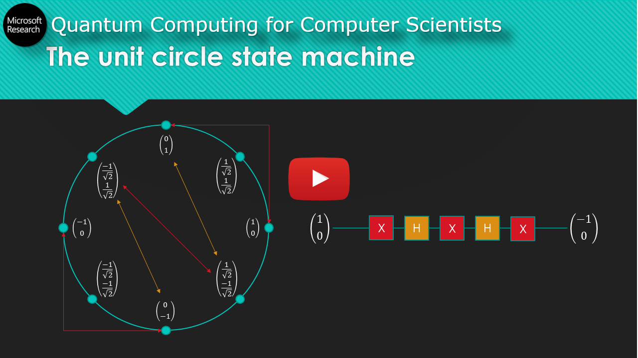
If you don’t know much about quantum logic gates or how a quantum computer works in general, I gave a talk aimed at computer scientists here (slides: pdf, pptx):

First, the good news: no compilation is necessary for our state vector. It works as-is. Things are quite a bit different for our Hamiltonian, however. We compile it by solving for \( U(t) \) in the following variant of the Schrödinger equation: $$ U(t) = e^{-i H t} $$ Where:

• \( U(t) \) is a matrix that takes time \( t \) as a parameter
• \( e \) is Euler’s number
• \( i \) is the imaginary number such that \( i^2 = -1 \)
• \( H \) is our Hamiltonian
• \( t \) is time (in seconds), a variable

There’s one very strange thing about this equation: it has a matrix as an exponent! What does that even mean?! How can you raise something to the power of a matrix? You can’t, at least not directly - you have to use an identity for \( e^x \) involving the Taylor series:

$$ e^x = \sum_{n=0}^{n=\infty} \frac{x^n}{n!} = 1 + x + \frac{x^2}{2!} + \frac{x^3}{3!} + \ldots $$

Plugging our Hamiltonian \( H \) into that identity moves it out of the exponent and into the (somewhat) more comfortable waters of an infinite sum:

$$ U(t) = e^{-iHt} = \sum_{n=0}^{n=\infty} \frac{(-iHt)^n}{n!} = 1 + (-iHt) + \frac{(-iHt)^2}{2!} + \frac{(-iHt)^3}{3!} + \ldots $$

which expands to:

$$ U(t) = 1 - i(Ht) - \frac{(Ht)^2}{2!} + \frac{i(Ht)^3}{3!} + \frac{(Ht)^4}{4!} - \frac{i(Ht)^5}{5!} - \frac{(Ht)^6}{6!} \ldots $$

Note that raising \(-1\) and \(i\) to successive powers follows the cycle \(1 \rightarrow -i \rightarrow -1 \rightarrow i \rightarrow 1\). Note also that for \(H = \sigma_z\), \(H^2 = \mathbb{I}\), the identity matrix, which is equivalent to the scalar \(1\). Thus the above sum becomes:

$$ U(t) = 1 - iHt - \frac{t^2}{2!} + \frac{iHt^3}{3!} + \frac{t^4}{4!} - \frac{iHt^5}{5!} - \frac{t^6}{6!} \ldots $$

To translate this into something we can use, we need the Taylor series expansions for sine and cosine:

$$ \sin(x) = x - \frac{x^3}{3!} + \frac{x^5}{5!} - \frac{x^7}{7!} + \ldots $$

$$ \cos(x) = 1 - \frac{x^2}{2!} + \frac{x^4}{4!} - \frac{x^6}{6!} + \ldots $$

We want to extract these infinite sums from our \(U(t)\) sum. This requires reordering the terms of our infinite sums, which if done carelessly can go extremely awry! Thankfully addition in infinite sums is commutative if the sum absolutely converges, which it does here, so we can do this. We can extract \(\cos(x)\) from the \(U(t)\) sum:

$$ U(t) = \cos(t) -iHt + \frac{iHt^3}{3!} - \frac{iHt^5}{5!} + \frac{iHt^7}{7!} + \ldots $$

From which it’s easy to extract \(\sin(x)\):

$$ U(t) = \cos(t) - iH \left( t - \frac{t^3}{3!} + \frac{t^5}{5!} - \frac{t^7}{7!} + \ldots \right) = \cos(t) - iH\sin(t) $$

Almost there! Now multiply both sides of the equation by the identity matrix and expand \(H\) to get:

$$ \begin{bmatrix}1 & 0 \\ 0 & 1\end{bmatrix}U(t) = \begin{bmatrix}1 & 0 \\ 0 & 1\end{bmatrix} \left( \cos(t) - i \begin{bmatrix} 1 & 0 \\ 0 & -1 \end{bmatrix}\sin(t) \right) $$ $$ U(t) = \begin{bmatrix}\cos(t) & 0 \\ 0 & \cos(t)\end{bmatrix} - \begin{bmatrix} i\sin(t) & 0 \\ 0 & -i\sin(t) \end{bmatrix} $$ $$ U(t) = \begin{bmatrix}\cos(t) - i\sin(t) & 0 \\ 0 & \cos(t) + i\sin(t)\end{bmatrix} $$

Recall the famous identity for Euler’s formula:

$$e^{ix} = \cos(x) + i\sin(x)$$

Plugging it in to our matrix, we finally have:

$$U(t) = e^{-iHt} = \begin{bmatrix} e^{-it} & 0 \\ 0 & e^{it} \end{bmatrix}$$

We successfully solved for \(U(t)\)! I wish we could say we are done, but not quite. \(U(t)\) must be the cumulative effect of our quantum logic circuit, but how do we actually build a circuit with that effect? Fortunately here it’s very simple; there’s a fundamental quantum logic gate called the Rz gate which almost exactly matches our \(U(t)\)! Here it is:

$$ Rz(\theta) = \begin{bmatrix} e^{-i \theta/2} & 0 \\ 0 & e^{i \theta/2} \end{bmatrix} $$

At long last, we end up with our compiled Hamiltonian!

$$ U(t) = Rz(2t) $$

Can you compile the Hamiltonian when it’s \(\sigma_x\) or \(\sigma_y\)?

Running the simulation

All the pieces are in place. Flip the switch and let it rip! Let’s see what our electron’s spin will be after, say, three seconds in the magnetic field:

$$ U(3)\begin{bmatrix} 1 \\ 0 \end{bmatrix} = Rz(2 \cdot 3)\begin{bmatrix} 1 \\ 0 \end{bmatrix} = \begin{bmatrix} e^{-i 6/2} & 0 \\ 0 & e^{i 6/2} \end{bmatrix}\begin{bmatrix} 1 \\ 0 \end{bmatrix} = e^{-i3}\begin{bmatrix} 1 \\ 0 \end{bmatrix} $$

Very exciting! I guess! What does this even mean? Actually, we’ve stumbled upon a very interesting phenomenon; to understand it, you’ll need to understand phase invariance. Basically, if two quantum states differ only by a phase (a scalar multiplier \(e^{i\theta}\)) then they are actually the exact same state. Multiple ways of writing the same thing. So, after three seconds in the magnetic field, our electron’s spin is unchanged. You may think this is a letdown, but actually we’ve discovered something very important: an eigenstate of our system!

Eigenstates are the system’s stable states. As an analogy, think of a compass in Earth’s magnetic field. The compass spins freely until pointing toward magnetic north. Once it points north, it’s in an eigenstate and won’t spin any further. That’s the situation here, except our “compass” (the electron’s spin) was already pointing “north”. Eigenstates are so-called because the state is an eigenvector of the Hamiltonian: multiplying the eigenvector by the Hamiltonian matrix is the same as just multiplying it by a scalar. We have the useful and important theorem that if something is an eigenvector of our Hamiltonian \(H\), it’s also an eigenvector of \(U(t) = e^{-iHt}\) (and vice-versa).

Eigenstates are very important. An electron in a specific atomic orbital is in an eigenstate. A fully-folded protein is in an eigenstate. Finding eigenstates is one of the main motivations for using Hamiltonian simulation. We found an eigenstate by accident, but there are algorithms you can use to search for them on purpose. Can you find a second eigenstate?

Enough about that - what about if we run our simulation on a start state that isn’t an eigenstate? How about running it for \(\pi/2\) seconds on our 50/50 up-down superposition state?

$$ Rz(2 \pi/2)\begin{bmatrix} \frac{1}{\sqrt{2}} \\ \frac{1}{\sqrt{2}} \end{bmatrix} = \begin{bmatrix} e^{-i \pi/2} & 0 \\ 0 & e^{i \pi/2} \end{bmatrix} \begin{bmatrix} \frac{1}{\sqrt{2}} \\ \frac{1}{\sqrt{2}} \end{bmatrix} = \begin{bmatrix} -i & 0 \\ 0 & i \end{bmatrix} \begin{bmatrix} \frac{1}{\sqrt{2}} \\ \frac{1}{\sqrt{2}} \end{bmatrix} = -i \begin{bmatrix} \frac{1}{\sqrt{2}} \\ \frac{-1}{\sqrt{2}} \end{bmatrix} $$

So our particle’s spin changes from the \(|+\rangle\) state to what’s called the \(|-\rangle\) state, picking up a global phase along the way. Fascinating! Of course, in reality you can’t just peek at the quantum state vector; you must destructively measure it. You can run this over and over to get a pretty good idea of the vector’s value, through a process called quantum tomography.

Upping the ante

Puzzled readers might be wondering where the promised quantum speedup comes in. It appears when the system you’re analyzing grows in size: if you’re analyzing a system with \(n\) properties (for example, \(n\) electrons each with their own spin) then the state vector is of size \(2^n\). If the properties in your system don’t affect each other then you can usually factor the exponential-sized state vector into a product of smaller vectors, but once the properties start affecting one another (entanglement) you have to bite the bullet and keep the full \(2^n\)-sized vector around. Quantum computers get this \(2^n\)-sized vector for free, simply because of how quantum mechanics works.

How it works in reality

Nobody ever stands at a chalkboard deriving the Hamiltonian of their system, outside of undergraduate physics classes. The most complicated Hamiltonian you can derive by hand is probably that of elemental Hydrogen, so this is all done numerically; scientists create a model of their system in a program like NWChem, then it sucks up a whole bunch of (classical) computing power before spitting out the Hamiltonian. Similarly, nobody stands around writing down Taylor series expansions and doing weird algebraic tricks to compile their Hamiltonian; there are (very complicated) compilation methods that work given certain properties about your Hamiltonian (for example using Q#’s Exp operator). Both the process of deriving and compiling a system Hamiltonian are fast-moving, active areas of research.

In conclusion

True credit to you if you made it this far, reader. That was a whole lot of math just to get the most absolutely basic, hello-world type example out the door. If you’re interested in learning more on this topic here are some resources I’ve found:

• The upcoming textbook Learn Quantum Computing with Python and Q# by Sarah C. Kaiser and Cassandra Granade has an entire chapter introducing quantum chemistry
• A talk by Robin Kothari on Hamiltonian simulation from a pure computer science perspective
• The review paper Quantum computational chemistry by McArdle et al. offers a significantly more technical overview of the material
• Chris Kang has written several introductory posts ([1] [2]) on Hamiltonian simulation

Posted for the Q# Advent Calendar 2019

Credit to Nathan Wiebe and Cassandra Granade for patiently helping me with the basics of Hamiltonian Simulation.