Two pictures of quantum computation -

Interpretations of quantum mechanics are boring. Boring! Maybe the universe has a strict partition between quantum and non-quantum. Maybe there are a bunch of parallel universes with limited crosstalk. Or maybe it’s whatever the Bohmian mechanics people are talking about. Shut up and calculate, I think. I don’t say this out of some disdain for idle philosophizing or to put on airs of a salt-of-the-earth laborer in the equation mines. It’s just there are so, so many interesting things you can learn about in quantum theory without ever going near the interpretation question. Yet it’s many peoples’ first & last stop. Rise above!

This one is about quantum interference. A humble phenomenon, usually first encountered in high school physics when learning about whether light is a particle or a wave. Maybe your physics teacher took your class down to the dark, empty, disused school basement and fired a laser through a grating. You saw an interference pattern on the wall that kinda resembled what you saw, with water, in the ripple tank back upstairs. And that was that.

Now, years later, maybe you’re a programmer who watched a video online where a nice man walks you through how quantum computers work (slides: pdf, pptx):

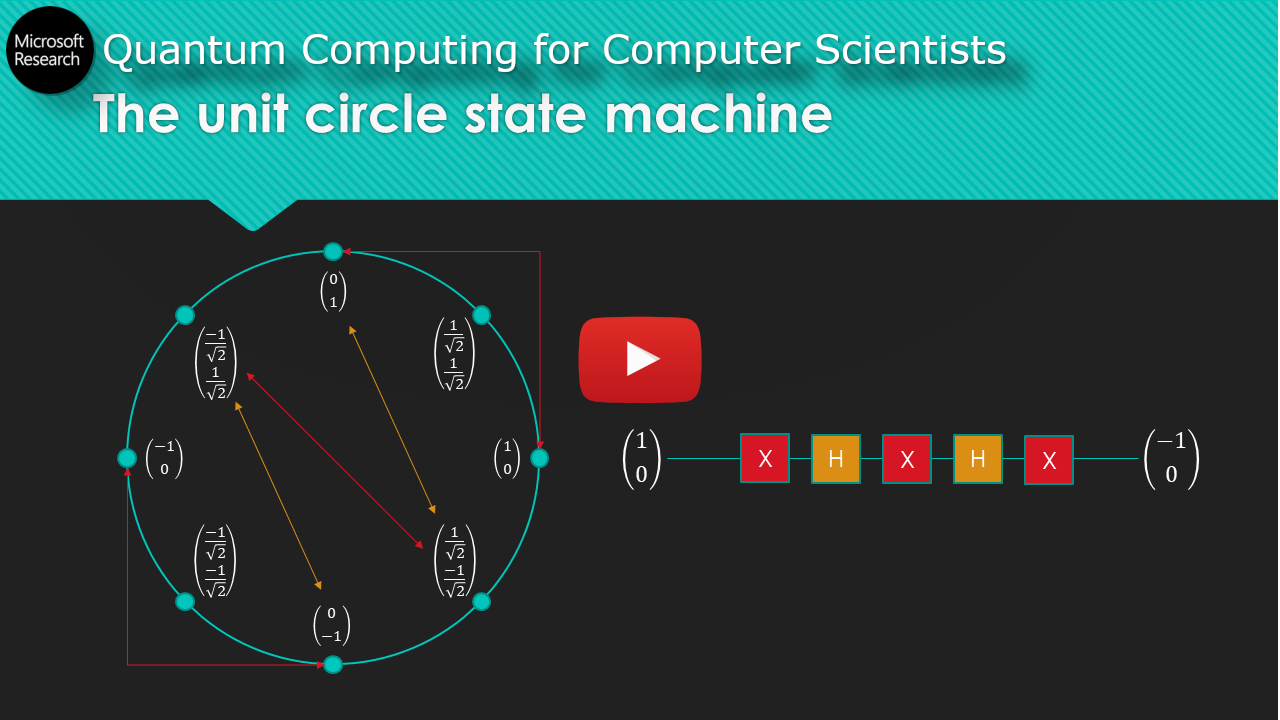
Preview of a slide from a quantum computing lecture, with a video play symbol superimposed.

It’s a state machine! Easy! Qbits are just pieces of state hopping around the unit circle. With a bit of linear algebra, the vault door protecting the treasures of quantum physics is flung open. Entanglement! Teleportation! Simulating physical reality! Breaking RSA! How polarized sunglasses work! Nothing withstands your intellectual onslaught. Until one day you’re reading a pop-science article about quantum computing, just to laugh at it of course, no tortured analogies for you because you KNOW. THE. MATH., and you see a learned physicist quoted as saying quantum computers make use of quantum interference. Quantum interference! That thing you learned about in high school… let’s see how it really works, with this unit circle state machine of ours. You run through a couple computations, looking for it.

It is nowhere to be found.

Textbook ambition

There’s a blog post out there called Prof. Sussman’s Reading List, where the professor has some fairly ambitious reading recommendations for high schoolers. If you have a university degree and have read them all I’ll count you a brighter person than I. One choice pick is Quantum Computing Since Democritus, a book by well-known complexity theorist Scott Aaronson. I started reading it after striking out with the Mermin relativity text. It’s a great read if you have a computer science degree - you know when you pick up a brand new textbook, all enthused & with the best of intentions, power through the first few chapters filled with material you already know, then take a break (never resumed) upon encountering the first concept requiring actual thought? Imagine if you could read a book that kept the feeling of those glorious early chapters most of the way through - that’s this book. It isn’t a book that’s good for learning the material. But if you already know the basic material, the book injects an enthusiasm, playfulness, and perspective that will have you thinking maybe complexity theory could really be for you.

Cover of the book Quantum Computing Since Democritus by Scott Aaronson. It features a portrait of Democritus pointing and laughing.

The book starts off with a fun dialogue from Democritus I can’t resist reproducing here:

Intellect: By convention there is sweetness, by convention bitterness, by convention color, in reality only atoms and the void.

Senses: Foolish intellect! Do you seek to overthrow us, while it is from us that you take your evidence?

Anyway. I held my own while reading this book up until chapter nine - actually I remember the exact paragraph & figure which shut down the run; talking about applying two Hadamard-like transformations to a qbit, it says:

“Intuitively, even though there are two “paths” that lead to the outcome $|0\rangle$, one of those paths has positive amplitude and the other has negative amplitude. As a result, the two paths interfere destructively and cancel each other out. By contrast, the two paths leading to the outcome $|1\rangle$ both have positive amplitude, and therefore interfere constructively.”

Strange diagram of a three-level binary tree with state 0 at the top, branching out into states 0 and 1, then state 0 branching again into states 0 and 1, and state 1 branching into states -0 and 1. The bottom 0 and -0 states are crossed out with a red X.

Needless to say I didn’t find this intuitive at all, whatsoever. It took me a long time to figure out exactly what was meant by this aside. And now I will share this hard-won knowledge with you, dear reader!

Negative probability? In my universe?

Aaronson presents quantum mechanics as a generalization of probability theory. We’re all familiar with how classical probability works - all the possible outcomes of an event have an associated probability between $0$ and $1$, and the sum of all of those probabilities must equal $1$. Imagine for a second you’re a supreme being designing your own universe. Maybe you want to tweak a few parameters. Perhaps - just to see what happens - you fiddle with your probability rules. Instead of probabilities summing to one, the sum of the squares of the probabilities sums to one. This is, essentially, how quantum mechanics works.

What are some implications of this rule change? The main one we’re interested in is how “probabilities” (let’s call them amplitudes from now on) can now be negative, since the square of a negative number is a positive number (if this confuses you go read the extended explanation in the QCSD lecture notes). What could it possibly mean for an event to have negative amplitude? As we’ll see below, an event with negative amplitude can cancel out an event with positive amplitude, ensuring it never happens! This is the basic idea underpinning destructive interference in quantum mechanics.

If you’re used to thinking about quantum computing the usual way, where vectors of amplitudes are transformed by matrix multiplication, you’ll miss this phenomenon. We need to see things differently! We need to use a different picture of quantum computation called sum-over-paths. As opposed to the standard (also called Schrödinger) approach where we keep a full vector of $2^n$ amplitudes around for $n$ qbits, in the sum-over-paths (also called Feynman) approach we focus on the final value of a single amplitude and trace all the different paths through the computation that contributed to it. How does it work?

Show me the math

Let’s look at a very basic example - applying the Hadamard operator twice to a single qbit, initialized to state $|1\rangle$. First, the standard approach with which we’re all familiar:

$$ HH|1\rangle = \begin{bmatrix} \frac{1}{\sqrt{2}} & \frac{1}{\sqrt{2}} \\ \frac{1}{\sqrt{2}} & \frac{-1}{\sqrt{2}} \\ \end{bmatrix} \begin{bmatrix} \frac{1}{\sqrt{2}} & \frac{1}{\sqrt{2}} \\ \frac{1}{\sqrt{2}} & \frac{-1}{\sqrt{2}} \\ \end{bmatrix} \begin{bmatrix} 0 \\ 1 \end{bmatrix} = \begin{bmatrix} \frac{1}{\sqrt{2}} & \frac{1}{\sqrt{2}} \\ \frac{1}{\sqrt{2}} & \frac{-1}{\sqrt{2}} \\ \end{bmatrix} \begin{bmatrix} \frac{1}{\sqrt{2}} \\ \frac{-1}{\sqrt{2}} \end{bmatrix} = \begin{bmatrix} 0 \\ 1 \end{bmatrix} = |1\rangle $$

Quantum interference is hidden somewhere in the calculations above, we just can’t see it! Let’s reveal it with the sum-over-paths method, which is easiest to understand recursively. Say we want to know the final value of amplitude $|0\rangle$ (the topmost one) after having applied the two Hadamard operators; we don’t care about any other amplitudes. Take a look at the final step in the computation again:

$$ \begin{bmatrix} \frac{1}{\sqrt{2}} & \frac{1}{\sqrt{2}} \\ \frac{1}{\sqrt{2}} & \frac{-1}{\sqrt{2}} \\ \end{bmatrix} \begin{bmatrix} \frac{1}{\sqrt{2}} \\ \frac{-1}{\sqrt{2}} \end{bmatrix} = \begin{bmatrix} 0 \\ 1 \end{bmatrix} $$

Zooming in on the only value we care about (the topmost element of the final vector), by the rules of matrix multiplication we can write this as follows:

$$ \frac{1}{\sqrt{2}} \cdot \frac{1}{\sqrt{2}} + \frac{1}{\sqrt{2}} \cdot \frac{-1}{\sqrt{2}} = 0 $$

Because of how matrix multiplication works, the final value of our amplitude $|0\rangle$ depends both on the previous value of amplitude $|0\rangle$ and the previous value of amplitude $|1\rangle$; both contribute. We can think of these two contributions as two paths coming together and (in this case) destructively interfering and canceling each other out! Also, our two paths really branch into four paths since this is the second of two Hadamard operators; here’s the full calculation linking all the way back to the initial state:

$$ \frac{1}{\sqrt{2}} \left( \frac{1}{\sqrt{2}} \cdot 0 + \frac{1}{\sqrt{2}} \cdot 1 \right) + \frac{1}{\sqrt{2}} \left( \frac{1}{\sqrt{2}} \cdot 0 + \frac{-1}{\sqrt{2}} \cdot 1 \right) = 0 $$

We could imagine, given a much larger series of gates acting on many qbits, how these paths could fan out recursively many times until they hit the initial state - then bubble back up, coming together at each fork to interfere constructively or destructively, accumulating in the final value of the amplitude we care about. Pretty neat! Okay, so we’ve found the missing interference. Now what? All we’ve done is rewrite matrix multiplication at greater length! Ah, but interference is just one of the prizes we’ve acquired.

Exponential burdens of another kind

With the standard picture of quantum computation we have to keep a $2^n$-sized vector of amplitudes around to model the behavior of $n$ qbits. Sure you can be clever and keep the qbits factored as long as possible, but once things get maximally entangled there’s no way around it. You need an exponential amount of space. This is a problem when you’re trying to simulate quantum computation on a classical computer. Classically simulating quantum computers is of interest not only to complexity theorists, but anyone who cares about the promise of quantum computation! If we figure out a way to efficiently (as in, with polynomial time/space overhead) simulate quantum computation on a classical computer, then we don’t have to bother with all the exotic nanofabrication and near-absolute-zero vacuum environments and whatnot. Just run your quantum program on the efficient classical simulator and send your condolences to the resultant horde of despondent grad students.

Now, currently there’s no good reason to believe that efficient quantum simulation is possible. That doesn’t mean we don’t have options. Like the one we’ve just learned about! It turns out the sum-over-paths picture is a classic time/space tradeoff. By recursively tracing these paths back through the computation, we never have to keep the entire state vector in memory; the (big!) downside is that our computation takes exponentially more time. Given $n$ qbits and $m$ gates, the standard picture uses $O(m2^n)$ time and $O(2^n)$ space, while the sum-over-paths picture uses $O(4^m)$ time and $O(n+m)$ space. How does it work?

Let’s define a recursive function $f(|\psi\rangle, U, i)$, where:

$|\psi\rangle$ is the initial state vector
$U$ is a list of operators to apply to $|\psi\rangle$, ordered from last to first
$i$ is the index of the amplitude we want to calculate

We’ll use linear algebra indexing conventions:

Indices count from $1$
For a vector, $|\psi\rangle[n]$ is amplitude $n$ in $|\psi\rangle$
For a matrix, $U[m,n]$ is the element in row $m$ and column $n$ of $U$

We have the following three recursive cases for $f(|\psi\rangle, U, i)$:

Base case: $U = [\ ]$, return $|\psi\rangle[i]$
General case: $U = [U_m, \ldots, U_{1}]$, where $U_m$ is a $2 \times 2$ matrix acting on 1 qbit; in the $i$th row of the full matrix $M = \mathbb{I}_2 \otimes \ldots \otimes U_m \otimes \ldots \otimes \mathbb{I_2}$ (which would be multiplied against the state vector), there will be at most two nonzero entries at some indices $a$ and $b$; this means we need the amplitudes at indices $a$ and $b$ from the state prior to $U_m$ being applied, so return:

$$ M[i,a]\cdot f(|\psi\rangle, Tail(U), a) + M[i,b] \cdot f(|\psi\rangle, Tail(U), b) $$

General case: $U = [U_m, \ldots, U_{1}]$, where $U_m$ is an operator acting on two qbits; in the $i$th row of the full matrix $M$ (which would be multiplied against the state vector), there will be at most four nonzero entries at some indices $a$, $b$, $c$, and $d$; this means we need the amplitudes at indices $a$, $b$, $c$, and $d$ from the state prior to $U_m$ being applied, so return:

$$ M[i,a]\cdot f(|\psi\rangle, Tail(U), a) + M[i,b] \cdot f(|\psi\rangle, Tail(U), b) + $$$$ M[i,c] \cdot f(|\psi\rangle, Tail(U), c) + M[i,d] \cdot f(|\psi\rangle, Tail(U), d) $$

We can apply this recursive algorithm to our example with the Hadamard operators up above:

$$ f(|1\rangle, [H, H], 1) = H[1,1] f(|1\rangle, [H], 1) + H[1,2] f(|1\rangle, [H], 2) $$ $$ f(|1\rangle, [H, H], 1) = \frac{1}{\sqrt{2}} f(|1\rangle, [H], 1) + \frac{1}{\sqrt{2}} f(|1\rangle, [H], 2) $$ $$ f(|1\rangle, [H, H], 1) = \frac{1}{\sqrt{2}} \left( \frac{1}{\sqrt{2}} f(|1\rangle, [\ ], 1) + \frac{1}{\sqrt{2}} f(|1\rangle, [\ ], 2) \right) + \frac{1}{\sqrt{2}} f(|1\rangle, [H], 2) $$ $$ f(|1\rangle, [H, H], 1) = \frac{1}{\sqrt{2}} \left( \frac{1}{\sqrt{2}} \cdot 0 + \frac{1}{\sqrt{2}} \cdot 1 \right) + \frac{1}{\sqrt{2}} f(|1\rangle, [H], 2) $$ $$ f(|1\rangle, [H, H], 1) = \frac{1}{2} + \frac{1}{\sqrt{2}} \left( \frac{1}{\sqrt{2}} f(|1\rangle, [\ ], 1) + \frac{-1}{\sqrt{2}} f(|1\rangle, [\ ], 2) \right) $$ $$ f(|1\rangle, [H, H], 1) = \frac{1}{2} + \frac{1}{\sqrt{2}} \left( \frac{1}{\sqrt{2}} \cdot 0 + \frac{-1}{\sqrt{2}} \cdot 1 \right) $$ $$ f(|1\rangle, [H, H], 1) = 0 $$

It’s easy to see how this algorithm would take $O(4^m)$ time; if there were $m$ 2-qbit operators, there would be four additional recursive calls at each level. An algorithmic hybrid of these two pictures exists which tries to use the best of each approach. It’s also fun to think about how you’d combine the pictures yourself, for example using memoization to avoid recalculating recursive calls with the same parameters.

Implementation in the Microsoft QDK

Microsoft’s Quantum Development Kit includes a very interesting simulation framework enabling developers to write their own classical simulator, then run their Q# programs on it! The QDK ships with three built-in simulators: a standard full-state simulator, a trace simulator to estimate resource usage (number of qbits etc.), and a Toffoli simulator to run reversible classical programs. We can write our own sum-over-paths simulator following the QDK simulator code samples. Unfortunately I ran out of time to actually write the simulator before this post’s publish date, but it seems like a nice Christmas holiday project so check back on this section in next couple of weeks! You can follow along with development at my repo here.

What about the picture?

Only one mystery remains. What’s the deal with this diagram? How do we semantically map our sum-over-paths algorithm to its tree structure?

The same interference diagram from up above.

I actually had a chance to ask Scott Aaronson about this directly in a HN AMA about two-and-a-half years ago, to give you an idea of how long this topic has been stewing in the back of my head. I didn’t really understand the answer; this diagram sort of works the exact opposite of how I understand sum-over-paths, because it branches out from the initial state instead of all the paths converging at the final state. I think we can probably rewrite our recursive algorithm as a bottom-up iterative algorithm based on depth-first search, in which case diagram makes a bit more sense. If you think you can explain this, I have an as-yet unanswered question on QCSE for this very topic. Any help would be much appreciated!

Two pictures of quantum computation

Quantum interference in the sum-over-paths formalism